The Kelly Criterion

What is it? Why is it interesting?

Consider a toy example of a gamble. Someone offers you a game where a fair coin will be tossed: you will win 70% of the money you bet when heads comes up and lose 60% of the money you bet when tails comes up. Furthermore, you are offered the opportunity to play this game many times, although not arbitrarily often, say just once a day. Intuitively, this gamble seems favorable, especially when you are allowed to play it repeatedly. However, it becomes trickier when you ask yourself questions like, “How much of my total wealth should I bet?” and “What is the best strategy to maximize my long-term wealth, say over 10 years?” The Kelly Criterion provides the answer to these questions!

To fully answer those questions, we need a few definitions and a bit of terminology (trust me, it will be worth the pain).

Let \(a > 0\) be the gain per unit of staked wealth on a win, and let \(0 < b \leq 1\) be the loss per unit of staked wealth on a loss. Furthermore, let \(0 < p < 1\) be the probability of winning. Then each gamble can be categorized as follows:

• Fair if \(a \cdot p = b \cdot (1 - p)\) .
• You have an edge if \(a \cdot p > b \cdot (1 - p)\) .
• You have a negative edge if \(a \cdot p < b \cdot (1 - p)\) .

Next, we introduce the fraction \(0 \leq f < \frac{1}{b}\) of your current wealth that you want to gamble. (Note: the upper bound \(1/b\) ensures \(1 - bf > 0\) so that log-returns remain finite; at exactly \(f=1/b\) a loss takes you to zero.)

To simplify the notation, whenever you bet a fraction \(f\) of your wealth:

\[ a_f = a \cdot f, \quad b_f = b \cdot f\]

---

Now suppose you repeat this game many times (potentially indefinitely). Denote your wealth at time \(t\) by \(X_t\) . This can be defined by

\[ X_{t+1} := X_t \cdot r_{t+1}, \]

where the \(r_t\) are i.i.d. and given by

\[ r_t = \begin{cases} 1 + a_f \text{ with probability } p, \\ 1 - b_f \text{ with probability } 1 - p. \end{cases} \]

A key question is:

\[ \text{Which } f \text{ maximizes } X_t(f) \text{ in the long run?}\]

A naive approach would be to look at the expected value \(E[X_t(f)]\) and choose \(f\) to maximize this expectation:

\[ \arg\max_{f} E[X_t(f)]\]

To see why this might lead to problems, we show that maximizing the expected value leads to always betting everything if we have an edge. If you bet fraction \(f\) of your wealth on this gamble, then:

• With probability \(p\) , your new wealth is \(X_0 \cdot (1 + a_f)\) .
• With probability \(1 - p\) , your new wealth is \(X_0 \cdot (1 - b_f)\) .

Taking the expectation of one bet and compounding it over \(t\) independent rounds gives

\[ E[X_t] = X_0 \bigl[1 + f \cdot \bigl(p \cdot a - (1 - p) \cdot b\bigr)\bigr]^{t}\]

Step-by-step expectation

The expected wealth after one bet is:

\[ E[X_1] = p \cdot X_0 \cdot (1 + a_f) + (1 - p) \cdot X_0 \cdot (1 - b_f)\]

Factoring out \(X_0\) gives:

\[ E[X_1] = X_0 \left[ p \cdot (1 + a_f) + (1 - p) \cdot (1 - b_f) \right]\]

Combine the terms inside the brackets:

\[ p \cdot (1 + a_f) + (1 - p) (1 - b_f) = p + p \cdot a_f + (1 - p) - (1 - p) \cdot b_f = 1 + f \bigl[p \cdot a - (1 - p) \cdot b\bigr]\]

Since the rounds are independent and each multiplies wealth by the same expected factor, the \(t\) -round expectation is that bracket raised to the power \(t\) .

As a function of \(f\) (over the interval \(0 \leq f \leq \frac{1}{b}\) ), this is a monotone expression. Consequently we can see that:

• If \(p \cdot a > b \cdot (1 - p)\) , then the coefficient of \(f\) is positive, and \(E[X_t]\) is maximized by choosing the largest possible \(f\) , meaning \(f = \frac{1}{b}\) (i.e., bet everything and even take leverage if possible).
• If \(p \cdot a < b \cdot (1 - p)\) , the coefficient of \(f\) is negative, so the maximum occurs at \(f = 0\) (i.e., do not bet at all).
• If \(p \cdot a = b \cdot (1 - p)\) , any \(f \in [0, \frac{1}{b}]\) yields the same expected wealth.

However, if you keep risking losing everything at each bet whenever \(p \cdot a > b \cdot (1 - p)\) , then with certainty you are going to go broke in the long run. This is analogous to the St. Petersburg paradox: maximizing expected value of a repeated multiplicative gamble can lead to ruin.

---

A more sophisticated approach is to optimize the Exponential Rate of Growth of your wealth \(X_t(f).\) Formally, we look for

\[ \arg\max_{f} G(f),\]

where

\[ G(f) := \lim_{t \to \infty} \frac{1}{t} \log \Bigl(\frac{X_t(f)}{X_0}\Bigr)\]

Assume that, out of \(t\) independent trials, \(W\) are wins and \(L\) are losses (with \(W + L = t\) ). Each win multiplies the current wealth by \((1 + a_f)\) , while each loss multiplies it by \((1 - b_f)\) . Therefore:

\[ X_t(f) = (1 + a_f)^W \cdot (1 - b_f)^L \cdot X_0\]

Taking logarithms leads to:

\[ G(f) = \lim_{t\to\infty} \Bigl[\frac{W}{t} \log \bigl(1 + a_f\bigr) + \frac{L}{t} \log \bigl(1 - b_f\bigr)\Bigr]\]

and noting that \(W/t \to p\) and \(L/t \to (1 - p)\) as \(t \to \infty\) , we get (under i.i.d. assumptions and by the strong law / ergodic theorem):

\[G(f) = p \log \bigl(1 + a_f\bigr) + (1 - p) \log \bigl(1 - b_f\bigr)\]

To find the optimal fraction \(f\) (the Kelly fraction), we set the derivative of \(G(f)\) with respect to \(f\) to zero and solve for \( f \) . The result is:

\[ f_{\text{Kelly}} = \frac{p}{b} - \frac{1 - p}{a}\]

Since \(G''(f) < 0\) on \(0 \le f < 1/b\) , the growth rate is strictly concave, so this maximizer is unique; if \(f_{\text{Kelly}} \le 0\) the constrained optimum is \(f^\star = 0\) .

Second derivative

\[ G''(f)=-\frac{pa^2}{(1+af)^2}-\frac{(1-p)b^2}{(1-bf)^2}<0 \]

Both terms are strictly negative for every \(0 \le f < 1/b\) , so \(G\) is strictly concave on its whole domain and can have at most one interior maximum.

If you do not have an edge, i.e. if

\[ p \cdot a \le b \cdot (1 - p),\]

then \(f_{\text{Kelly}} \le 0\) , meaning you should not bet at all. Conversely, when you do have an edge (\(p \cdot a > b \cdot (1 - p)\) ), the Kelly criterion gives a positive fraction to bet, balancing the risk of ruin against potential growth to maximize your wealth’s long-term growth rate.

Below I show a plot for the parameters \( p=0.7,\ a = 1.5,\ b = 0.95 \) , which are deliberately more favourable than the coin-flip we opened with; dial the sliders to \(p = 0.5\) , \(a = 0.7\) , \(b = 0.6\) to recover that example. Please notice that even if you bet everything in this favorable game your growth rate can become negative if you risk all your wealth on a single bet!

History

One might assume that ideas like the Kelly Criterion would naturally emerge in the context of investing or casino gambling. However, its first rigorous derivation arose from a somewhat different problem.

In 1956, J. L. Kelly Jr., a researcher at Bell Labs, studied gambling with side information conveyed over a noisy channel. He showed that maximizing expected log capital growth yields a long‑run growth rate equal to the mutual information rate between the side information and outcomes; the optimal bets use the conditional probabilities given that information. This establishes a clean bridge from Shannon’s channel capacity to optimal capital growth in uncertain environments. For more details, see Kelly’s original paper, “A New Interpretation of Information Rate” (link below).

Ergodicity (‑breaking)

This section can be skipped without losing much information about the Kelly Criterion. Nevertheless I included it, because I think that ergodicity, though not directly connected to the Kelly Criterion, is closely related and even a generalization of the phenomenon where the arithmetic properties of a random process differ from the geometric ones. In particular, it sheds light on the distinction between an ensemble and a single realization of a process.

Informally, a random process \( X_t \) is called ergodic if its time average of any well-behaved function equals the corresponding ensemble average (expectation). In discrete time, this often appears as:

\[ \lim_{T \to \infty} \frac{1}{T} \sum_{t=1}^{T} g\bigl(X_t\bigr) = \mathbb{E}\bigl[g(X_t)\bigr], \]

for any integrable function \(g\) . Equivalently, “time averages” along one infinitely long sample path converge to the “ensemble average” across all possible sample paths.

A non-ergodic process is one where at least one function \(g\) violates the above equality, meaning the time average and the ensemble average do not match.

---

Next we look at a toy example of an ergodic process: the simple coin flip. At each discrete step \( t \) , flip a coin which lands with \( 60\% \) heads up and \( 40\% \) tails up. If it lands on heads, you win \( +1 \) and if it lands on tails, you lose \( -1 \) . This means you have a positive arithmetic edge. So the per-flip increment is \( X_t \in \{ +1, -1 \} \) with probability \( 0.6 \) and \( 0.4 \) respectively, and the simulation below plots the cumulative sum of those increments. The ensemble average of one flip is \( 0.2 \) . The time average of a long sequence converges to the same \( 0.2 \) (by the Law of Large Numbers), showing ergodicity.

Below is a live simulation of this process: every individual path’s own long-run slope converges to the same slope as the ensemble average, since the process is ergodic.

For an example of a non-ergodic toy process we look at multiplicative growth. A wealth at time \( t \) denoted by \( X_t \) evolves multiplicatively:

\[ X_{t+1} = X_t \cdot r_{t+1},\]

where \( r_{t+1} \) is a random factor. In this example, let: \( r_{t+1} \in \{ 1.7, 0.5 \} \) with probability \( 0.5 \) each, and \( X_0 = 1 \) . The ensemble average at time \( t \) is

\[ E[X_t] = \left(0.5 \cdot 1.7 + 0.5 \cdot 0.5\right)^t = 1.1^t\]

However, because the geometric mean of the per‑period factor is below \( 1 \) ,

\[ \exp\Big(0.5 \cdot \log(1.7) + 0.5 \cdot \log(0.5)\Big) \approx 0.92 < 1,\]

the single-path behavior drifts to \(0\) in the long run. In fact,

\[ \lim_{t\to\infty}\frac{1}{t}\log X_t = E[\log r] = \tfrac12\log(1.7)+\tfrac12\log(0.5) < 0 \quad\text{almost surely}, \]

so \(X_t \to 0\) a.s., even though the ensemble average grows like \( 1.1^t \) . Hence:

\[ \text{time average} \neq \text{ensemble average} \rightarrow \text{non-ergodic}\]

Below is a live simulation of this process. Try setting \(f=1\) (bet everything each round) with the default win/loss multipliers: the ensemble average (green dashed line) climbs steadily, yet almost every individual path drifts toward zero.

This example illustrates what happened in our introductory example. Even though the edge was clearly positive (which is reflected in the ensemble average, the dashed green line), a single realization of the multiplicative process approaches zero most of the time.

Kelly as a potential solution for non-ergodic multiplicative growth

The “Ergodicity Problem” refers to situations where researchers incorrectly apply ensemble averages to systems where the time average is the relevant measure. This often leads to misleading conclusions, especially in systems where the time average and the ensemble average do not align. The problem can also occur in reverse, when researchers focus on time averages in processes where ensemble averages would be more appropriate. In non-ergodic systems, the time average can differ significantly between individual realizations of a random process.

In the specific case of multiplicative growth processes, the Kelly Criterion offers a compelling solution to the ergodicity problem. The Kelly Criterion maximizes the long-term multiplicative growth rate of wealth by optimizing the geometric mean of returns. This is mathematically equivalent to maximizing the time average of a multiplicative growth process, as will be shown below. Furthermore, it can be demonstrated that the multiplicative growth rate (or any well-defined growth rate) is an example of an ergodic observable, one where the time average converges to the ensemble average.

For more on the ergodicity problem and ergodic observables, I highly recommend exploring the blog posts and scientific papers by Ole Peters (link provided below).

Investing

The Kelly Criterion and its variations naturally arise in investing. Since investing is all about multiplicative growth and every person has only one life to roll the dice, it is critical to tame randomness as much as possible, especially when the odds are favorable.

Practical notes. Real systems impose leverage/margin constraints that cap \(f\) and may liquidate positions before \(1-bf=0\) . Parameter uncertainty (e.g., estimating \(p,a,b\) ) often motivates fractional Kelly (e.g., half-Kelly) in practice.

Safe haven investing

One book that brings together ideas about multiplicative growth, ergodicity, the Kelly Criterion, and insurance strategies in investing is Safe Haven by Mark Spitznagel. As this book was a key inspiration for me to write this blog post, I highly recommend it to anyone interested in these topics (link provided below).

In this post, I won’t delve into the primary focus of the book, which investigates how investing with an “insurance” component can potentially yield a higher multiplicative growth rate than even the Kelly Criterion. Instead, I’d like to emphasize several subtle points from the book that deserve a closer examination. Before this I want to state the definitions of the geometric mean and the median in discrete and continuous settings, because they are needed:

Geometric Mean \( GM \) :

\[ GM = \exp \left( \sum_{i} p(x_i) \cdot \log (x_i) \right), \quad GM = \exp \left( \int_{0}^{\infty} \log (x) \cdot p(x) dx \right)\]

Median \( m \) :

\[ \sum_{x_i \leq m} p(x_i) = \frac{1}{2}, \quad \int_{0}^{m} p(x) dx = \frac{1}{2}\]

Now the interesting statements:

1. Optimizing the multiplicative growth rate is equivalent to optimizing the geometric mean of the ending distribution of the process and equivalent to optimizing expected logarithmic utility of the process.

2. Optimizing the geometric mean of the ending distribution of the process is mathematically equivalent to optimizing the median of the ending distribution of the process.

3. To optimize other quantiles, such as the 5th percentile (\(q_{0.05}\) ), one can use the fractional Kelly Criterion. This approach involves betting a fraction \(\alpha\) of the full Kelly bet, where \(\alpha < 1\) . For example, using \(\alpha = \tfrac{1}{4}\) results in a betting fraction of:

\[ f = \frac{1}{4} \cdot f_{\text{Kelly}}\]

This fractional strategy balances growth and risk, allowing for targeting specific quantiles of the wealth distribution.

In the next section, I will clarify these points and show that, while they are approximately true (as stated in the book), they are not entirely correct when taken together. Specifically:

• Point (1) is always valid.
• Point (2) holds only in the limit as \(t\) approaches infinity (and even then via an approximate lognormal description).
• Point (3) applies when \(t\) is finite, and the exact fraction of Kelly that maximizes a given quantile depends on \(t\) .

This implies that (2) and (3) become somewhat contradictory if you try to apply them at the same time.

Subtleties in infinity

In the coming sections we look at the multiplicative growth process of wealth \( X_t \) and use the same notation as before.

Equivalences

Three objectives get used interchangeably in this literature: the exponential growth rate \(G(f)\) , the expected logarithmic utility \(\mathbb{E}[\log X_t(f)]\) that Bernoulli proposed for the St. Petersburg paradox, and the geometric mean \(GM(X_t(f))\) . They are all monotone transforms of the same quantity, \(\mathbb{E}[\log X_t(f)] = \log X_0 + t\,\mu(f)\) : dividing by \(t\) gives the growth rate, exponentiating gives the geometric mean, and neither operation moves an \(\arg\max\) . So the three agree on the optimal \(f\) , and they agree for every \(t\) , not just asymptotically.

The three objectives written out

\[ G(f) = \lim_{t \to \infty} \frac{1}{t} \log \Bigl(\frac{X_t(f)}{X_0}\Bigr), \qquad \arg\max_{f} \mathbb{E} \left[ \log (X_t(f)) \right], \qquad \arg\max_{f} GM(X_t(f))\]

Every one of them is built from \(\log (X_t(f))\) . The geometric mean simply wraps it in the exponential, which is strictly increasing and therefore leaves the maximizing \(f\) unchanged.

Infinite Case

Here we look at the case of \( t \rightarrow \infty \) . It helps to look at the distribution of the process as \( t \) gets bigger. Since the process is multiplicative and the random factors are i.i.d., the Central Limit Theorem implies that \(\log X_t\) is approximately normal for large \(t\) . Concretely (including the \(f\) -dependence explicitly):

\[ \log (X_t) = \log (X_0) + \sum_{n=1}^t \log (r_n(f)) \]

Define \( Y := \log (r(f)) \) with

\[ \mu (f) = \mathbb{E} \left[ Y \right], \qquad \sigma^2 (f) = \operatorname{Var}( Y ) \]

By the CLT the sum \(\sum_{n=1}^t Y_n\) is approximately normally distributed with parameters

\[ t \cdot \mu (f), \quad t \cdot \sigma^2 (f) \]

Therefore \( X_t \) is approximately lognormal with parameters

\[ \log (X_0) + t \cdot \mu (f), \quad t \cdot \sigma^2 (f) \]

---

Now we take a look at which fractions \( f \) will optimize specific quantiles of the large-\(t\) (approximately lognormal) distribution. By the Central Limit Theorem,

\[ \log X_t \approx \log X_0 + t \cdot \mu(f) + \sqrt{t} \cdot \sigma(f) Z, \qquad Z \sim N(0,1) \]

Writing \(z_q\) for the \(q\) -quantile of a standard normal and exponentiating gives the \(q\) -quantile of wealth itself,

\[ Q_q(X_t) \approx X_0 \exp \Bigl(t \cdot \mu(f) + \sqrt{t} \cdot \sigma(f) z_q\Bigr) \]

Maximizing that over \(f\) leads to the first-order condition

\[ \mu'(f) + \frac{z_q}{\sqrt{t}} \sigma'(f) = 0 \]

This is the whole story in one line. The quantile you happen to care about enters only through the term \(z_q/\sqrt{t}\) , and that term vanishes as \(t \to \infty\) , leaving \(\mu'(f) = 0\) .

Quantile derivation

Let \(q \in (0,1)\) and let \(Q_q(X_t)\) denote the \(q\) -quantile of \(X_t\) , that is the number \(x\) with

\[ \mathbb{P}\bigl(X_t \le x\bigr) = q \]

Because \(\log\) is strictly increasing, quantiles carry over to the log domain unchanged:

\[ Q_q\bigl(\log (X_t)\bigr) = \log \Bigl(Q_q(X_t)\Bigr) \]

Applying the normal approximation and the definition of \(z_q\) ,

\[ Q_q\bigl(\log X_t\bigr) \approx \log X_0 + t \cdot \mu(f) + \sqrt{t} \cdot \sigma(f) z_q \]

So maximizing the quantile means maximizing the exponent,

\[ \arg \max_f \Bigl[ t \cdot \mu(f) + \sqrt{t} \cdot \sigma(f) z_q \Bigr] \]

Differentiating with respect to \(f\) and setting the result to zero,

\[ t \cdot \mu'(f) + \sqrt{t} \cdot z_q \sigma'(f) = 0, \]

and dividing through by \(t\) gives the first-order condition quoted above.

That means the optimal \(f\) for any fixed quantile \(q\) converges to the same value \(f_{\text{Kelly}}\) that maximizes \( \mu(f) \) , the expected logarithmic utility and in turn \( G(f) \) , the exponential rate of growth. In other words, the Kelly fraction becomes optimal for all quantiles as \(t \to \infty\) .

As this derivation is very tedious, I want to make sure that you get the intuition right. As \( f \) increases up to the optimal fraction \( f_{\text{Kelly}} \) , both the growth rate and the variance of the distribution increase. Going further beyond the Kelly fraction gets dangerous: the growth rate declines while the variance still increases! This is the reason why practitioners often recommend being on the safe side of the optimal fraction. Generally, in a finite setting (as the next section illustrates) this can lead to lower quantiles being optimized by fractional Kelly bet sizes lower than the optimal fraction and higher quantiles being optimized by multiples of the optimal fraction. However, as \( t \to \infty \) the optimal growth rate dominates the variance effects and becomes optimal for all quantiles.

Finite Case

Now we look at the case when \( t \) stays finite. An analytical treatment would require the exact distribution of \( X_t \) , which depends on the full law of \( r_t \) , so we use simulations instead.

It is worth being precise about what the second claim actually asserts, because it is easy to refute the wrong statement. The claim is about maximizers: that the \(f\) maximizing the median coincides with the \(f\) maximizing the geometric mean. It is not the weaker statement that the two quantities are numerically equal. Showing median \(\neq\) GM at some finite \(t\) therefore proves nothing on its own, since two different objectives can still share an \(\arg\max\) .

The sharp version is this. The median and the geometric mean coincide exactly whenever \(\log X_t\) is symmetric about its mean, lognormality being one sufficient case among many. For \(p = 1/2\) , which covers both the coin flip we opened with and the ergodicity example, \(\log X_t\) is a shifted binomial with equal weights and so is symmetric for every finite \(t\) . In that case median \(=\) GM exactly, and the median-maximizing fraction is precisely \(f_{\text{Kelly}}\) at any horizon.

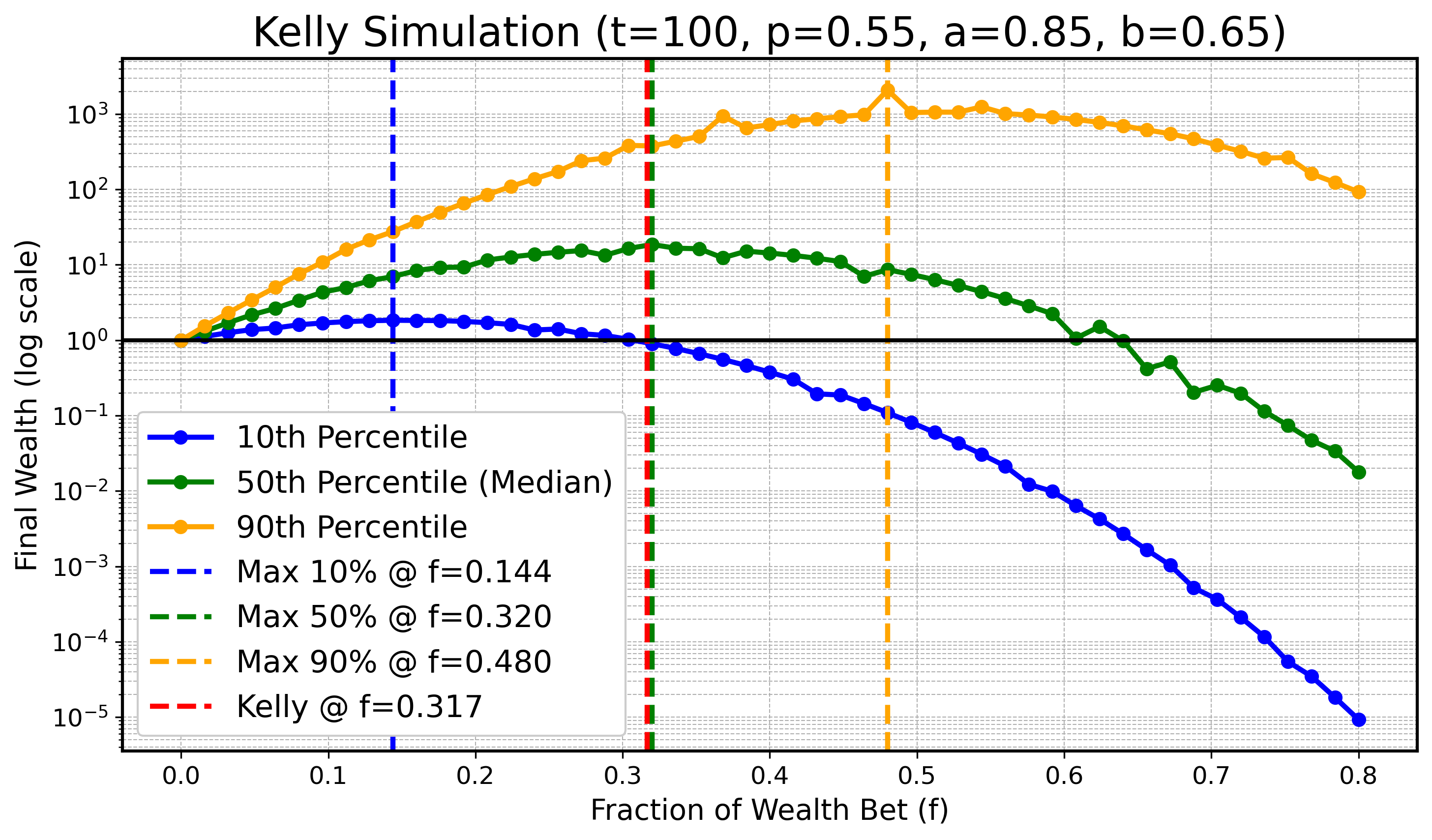
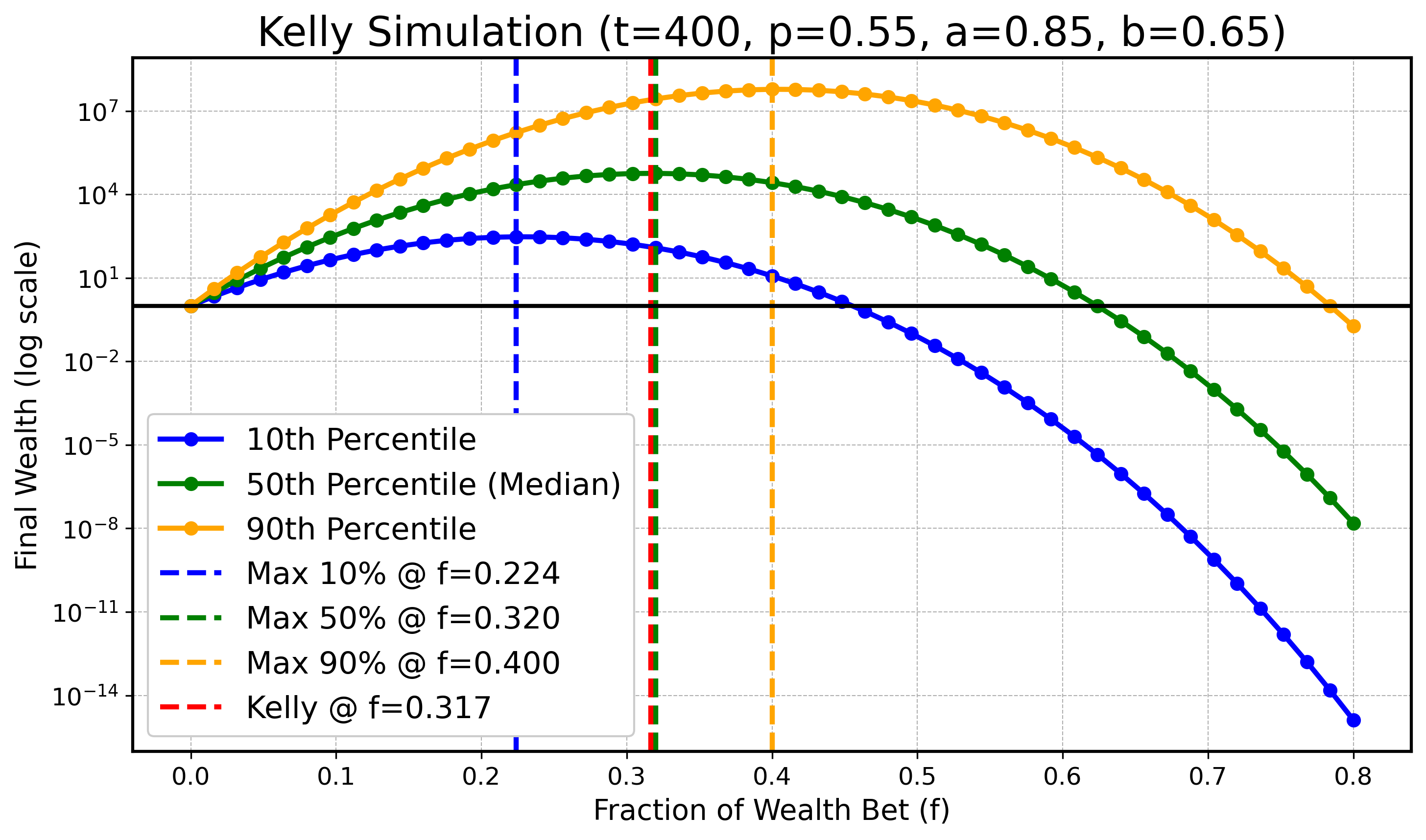
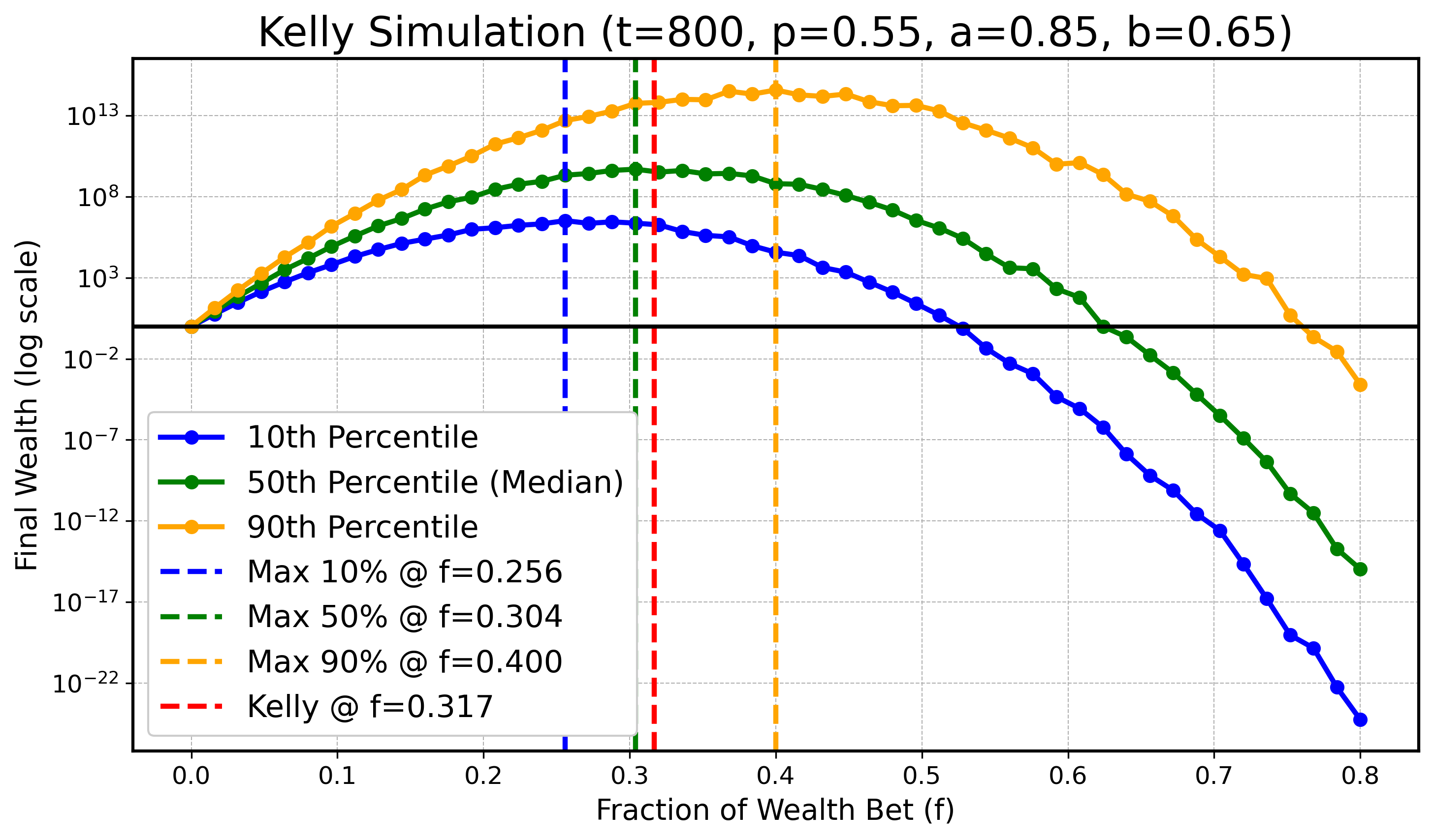
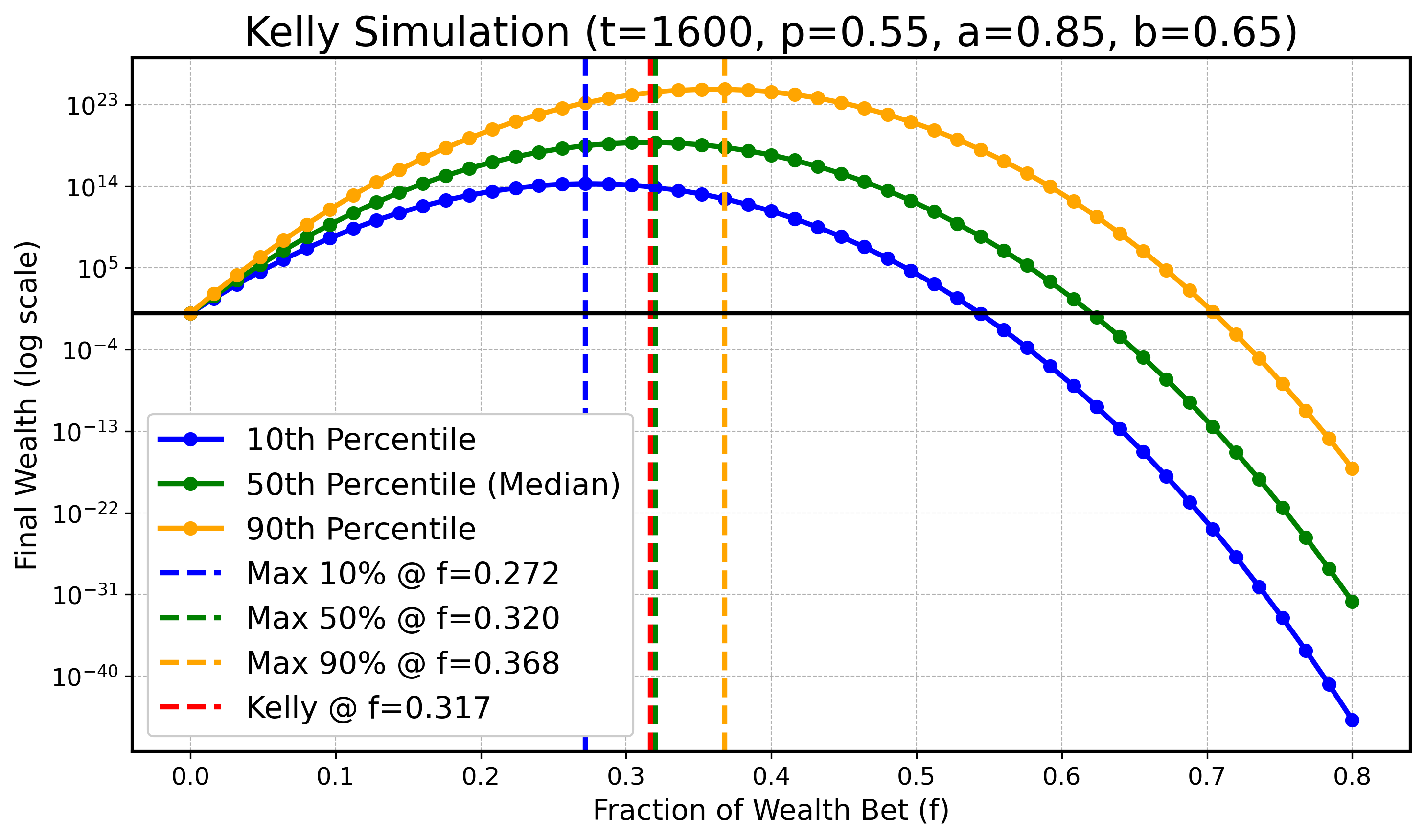
For \(p \neq 1/2\) the distribution is skewed, the two quantities genuinely differ, and, more to the point, their maximizers can differ too. The simulation below uses \(p = 0.55\) and shows exactly that.

We will do a simulation to illustrate that for finite \( t \) the optimum for lower or higher quantiles might be smaller/bigger than \( f_{\text{Kelly}} \) , however as \( t \) gets bigger these optimal values for quantiles converge to \( f_{\text{Kelly}} \) . Specifically we will look at \( X_t \) defined as before with parameters:

\[ a=0.9, \quad b=0.6, \quad p=0.55, \]

and \( t \in \{ 100, 200, 400, 800, 1600, 3200 \}. \) In all following plots we will draw the theoretical optimal fraction in red, \( f_{\text{Kelly}} \) , and also draw the optimal fractions of \( q_{0.1} \) , \( q_{0.5} \) (the median), and \( q_{0.9} \) in blue, green, and orange as dashed vertical lines respectively.

\(t = 100\) :

\(t = 200\) :

\(t = 400\) :

\(t = 800\) :

\(t = 1600\) :

\(t = 3200\) :

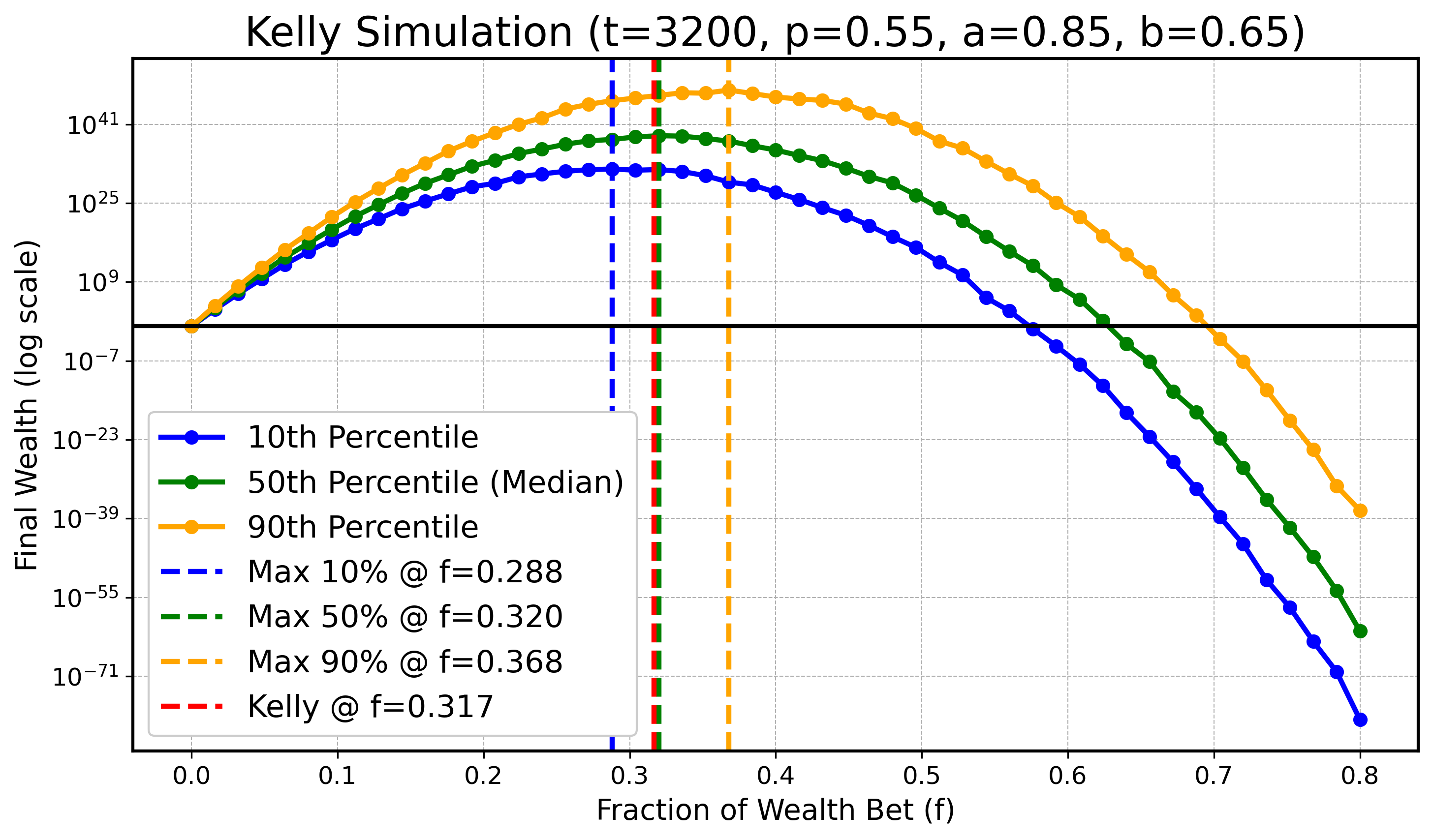
Although with slight numerical inaccuracies due to limited simulation resources, one can clearly see the trend as \( t \) gets bigger that the maximizing fractions for the 10th and 90th quantiles get closer to the optimizing median fraction and the theoretical optimal fraction \( f_{\text{Kelly}} \) .

Conclusion

The goal of this blog post was to introduce the Kelly Criterion with as much intuition as possible while maintaining the necessary rigor. While the derivation and explanation of the Kelly Criterion itself are not unique and can be found in many other resources, I strongly recommend reading the original paper to appreciate its historical and contextual significance.

In addition to introducing the Criterion, I sought to place it within the broader context of ergodicity, a fascinating topic that provides a deeper understanding of the Kelly Criterion and its practical applications.

The primary motivation for this post, however, stems from the nuanced and thought-provoking arguments presented in Mark Spitznagel’s Safe Haven. My aim was to clarify the subtle distinctions between the infinite and finite cases of the Kelly Criterion, which can be difficult to grasp and for which clear explanations are often lacking online. I hope my arguments help illuminate these concepts and address common points of confusion.

Key Takeaways:

1. Unified Optimization Optimizing the exponential rate of growth \(G(f)\) , the expected logarithmic utility of wealth \( \mathbb{E} \big[ \log(X_t(f)) \big] \) , and the geometric mean \( \text{GM}(X_t(f)) \) all lead to the same maximizer: \( f_{\text{Kelly}} \) .

2. Median vs. Geometric Mean The median of the wealth distribution \( X_t \) coincides with its geometric mean exactly when \(\log X_t\) is symmetric about its mean, which includes the symmetric case \(p = 1/2\) at every finite \(t\) . Otherwise the two agree only asymptotically, where by the CLT the distribution is approximately lognormal.

3. Finite vs. Infinite Horizons This is the most crucial point: A fractional Kelly strategy (i.e., betting a fraction of \( f_{\text{Kelly}} \) ) only optimizes a lower quantile of the wealth distribution for a finite time horizon \(t\) . As finite beings, this is arguably acceptable. However, the optimal fraction of \( f_{\text{Kelly}} \) depends heavily on \(t\) .

   • As \( t \to \infty \) , this fraction converges to 1, meaning \( f_{\text{Kelly}} \) becomes optimal for all quantiles.
   • This is an encouraging result for gamblers and investors: the longer you play the game, the less it matters which quantile you aim to optimize.
   • Nevertheless, it’s important to note that betting below \( f_{\text{Kelly}} \) often results in better outcomes in finite cases, as it reduces the variance in wealth.

I hope this post provides both clarity and practical insights into the Kelly Criterion, its applications, and its implications for decision-making over finite and infinite horizons.

Sources

• Source code for all simulations in the post can be found under: github
• Original Paper from J. L. Kelly Jr.
• Blog from Ole Peters: blog
• Safe Haven by Mark Spitznagel